COMSOL agent workflow: reproducing an HBM h-BN study with Codex

We took a fresh arXiv paper on GPU-HBM thermal design, opened COMSOL, and let an AI agent for COMSOL build the first reproducible simulation harness while the Desktop stayed visible.

In ChatGPT terms, this is the COMSOL agent people keep asking for: connect to a live COMSOL Desktop, build a model, run sweeps, capture figures, and leave scripts plus command traces behind.

The paper is arXiv:2510.11461, a COMSOL study of a 3D GPU-memory stack with a boron nitride interposer. The manuscript reports the important physics, material contrast, cooling coefficients, and sweeps, but it does not publish an `.mph` file, exact package dimensions, mesh, TSV details, or raw tables. So this is a trend-level reproduction log: a named COMSOL project, scripts, screenshots, and numeric traces that can be tightened if the missing geometry arrives.

Animated overview moving from arXiv paper figures to COMSOL shared Desktop automation and result plots. — Short video overview of the loop: one compact source-paper frame for context, then a COMSOL-heavy automation path: live attach, CLI control, geometry, selections, sweep, COMSOL rendering, and Python postprocess. Paper excerpts are adapted from Wang, Yan, and Huang's arXiv:2510.11461 under CC BY 4.0; they are cropped and composited here. A GIF fallback is also available.

COMSOL shared Desktop on the left and Codex on the right after model identity checkpointing. — Step one: bind Codex to COMSOL through sim's shared Desktop mode, then save a named `.mph` checkpoint before any serious geometry work. This display image is cropped and lightly sharpened; the raw full capture is preserved.

Control Path

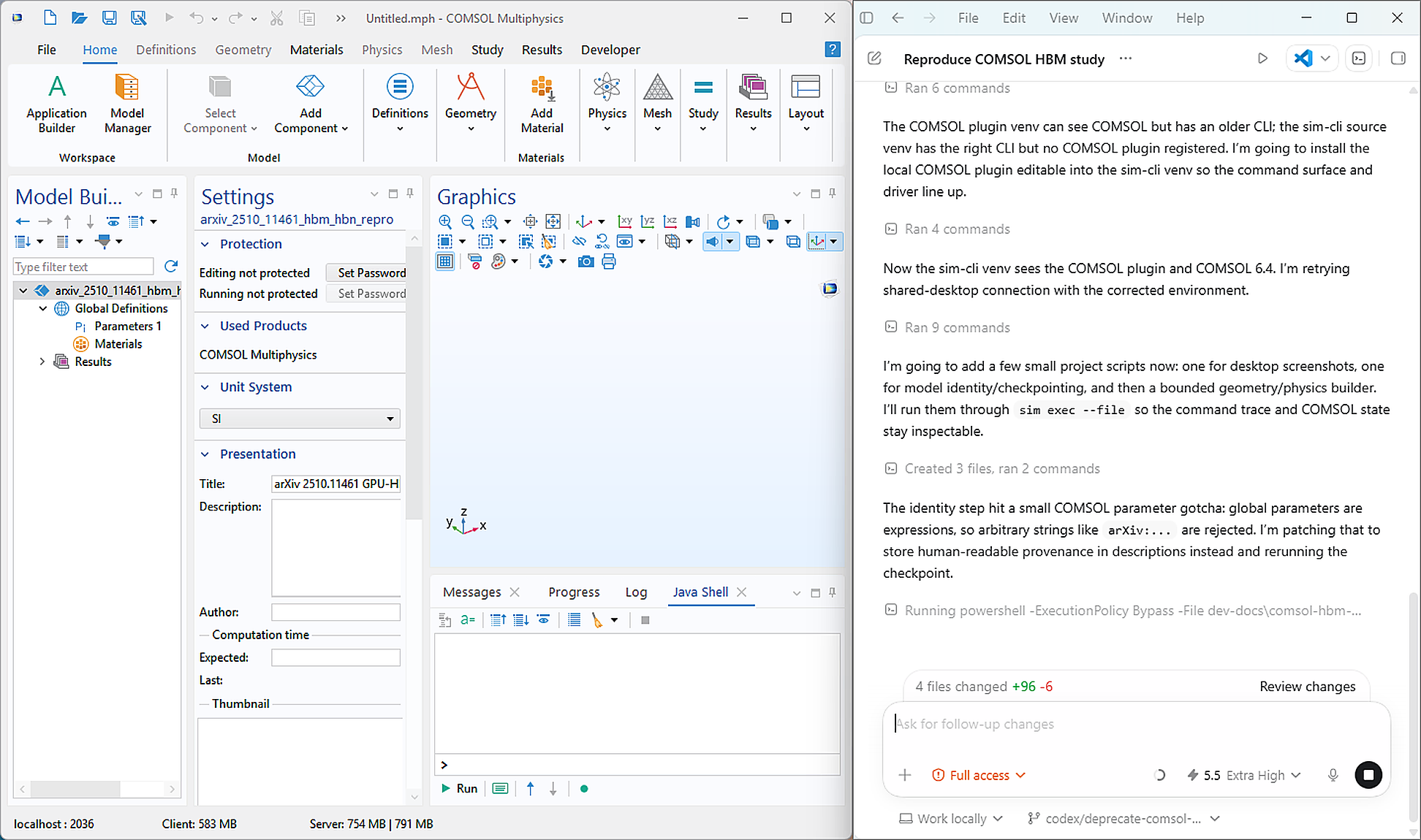
We ran COMSOL through `sim-cli` in shared Desktop mode, which starts `comsolmphserver`, attaches COMSOL Desktop to that same server, and lets Codex work against the Desktop's active model tag. That gave us a live Model Builder view while keeping every geometry edit, solve, and export reproducible from script.

uv pip install --python .\.venv\Scripts\python.exe -e ..\sim-plugin-comsol
.\.venv\Scripts\python.exe -m sim connect --solver comsol --ui-mode gui --driver-option visual_mode=shared-desktop
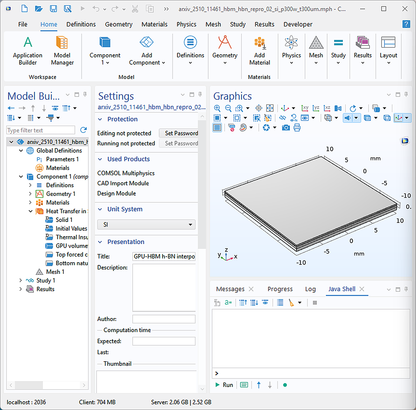
.\.venv\Scripts\python.exe -m sim --session b68f93bc-c84f-4ae4-8bb2-6d9a0ab40f6f inspect session.health

The health check reported `effective_ui_mode: shared-desktop`, `model_builder_live: true`, and `active_model_tag: Model1`. That made the screenshots honest: the COMSOL tree we watched was the model the scripts were mutating.

What Broke

This was not a clean one-shot automation run. The stationary COMSOL solves did not diverge, but the workflow had several very normal engineering failure modes:

Driver environment mismatch. One virtualenv could see COMSOL but had an older `sim` command surface; the newer `sim-cli` checkout had the right CLI but no COMSOL plugin installed. The fix was installing the local COMSOL plugin into the `sim-cli` env, then reconnecting and verifying `session.health`.
COMSOL parameter values are expressions. I first tried to store `arXiv:2510.11461` as a global parameter value. COMSOL rejected it because parameters are parsed as numeric expressions, not arbitrary strings. Provenance moved into labels and descriptions; parameter values stayed numeric.
Selections needed API probing. Box selections for boundaries were easy to make but easy to make empty. Setting `entitydim` explicitly, then checking `sel.entities()` before assigning materials and heat fluxes, kept the model from silently solving the wrong domain.
The public plot path changed. COMSOL result nodes were useful for model state, but the exported GUI screenshot was not a good public visualization. The final blog plots come from Python reading CSV/JSON result traces, which made the comparison clearer and repeatable.

Cropped COMSOL graphics view showing the representative stacked GPU interposer thermal geometry. — The first representative geometry: substrate, interposer, GPU heat-source die, and heat spreader. This cropped detail comes from the full side-by-side capture; COMSOL-generated selections gave stable domain names for materials and heat sources.

Model Built

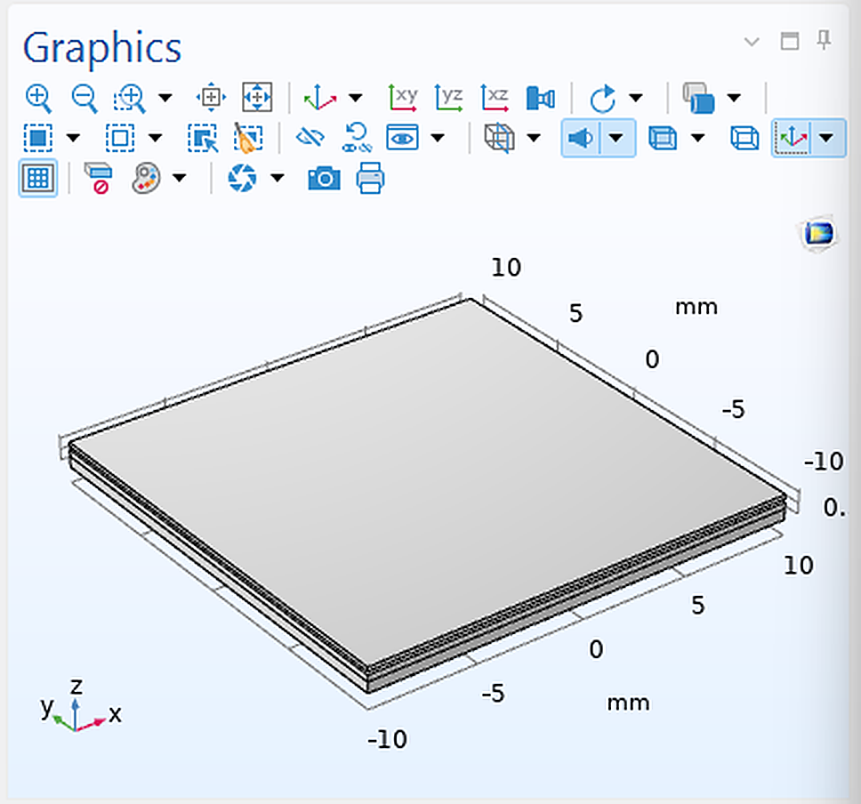
The first harness is intentionally compact: a 20 mm square stack, a 300 µm interposer, a central GPU heat source, top forced convection, and bottom natural convection. Silicon and copper are isotropic. h-BN is anisotropic, with high in-plane conductivity and lower through-plane conductivity. The script writes checkpointed `.mph` files and JSON result traces after every case.

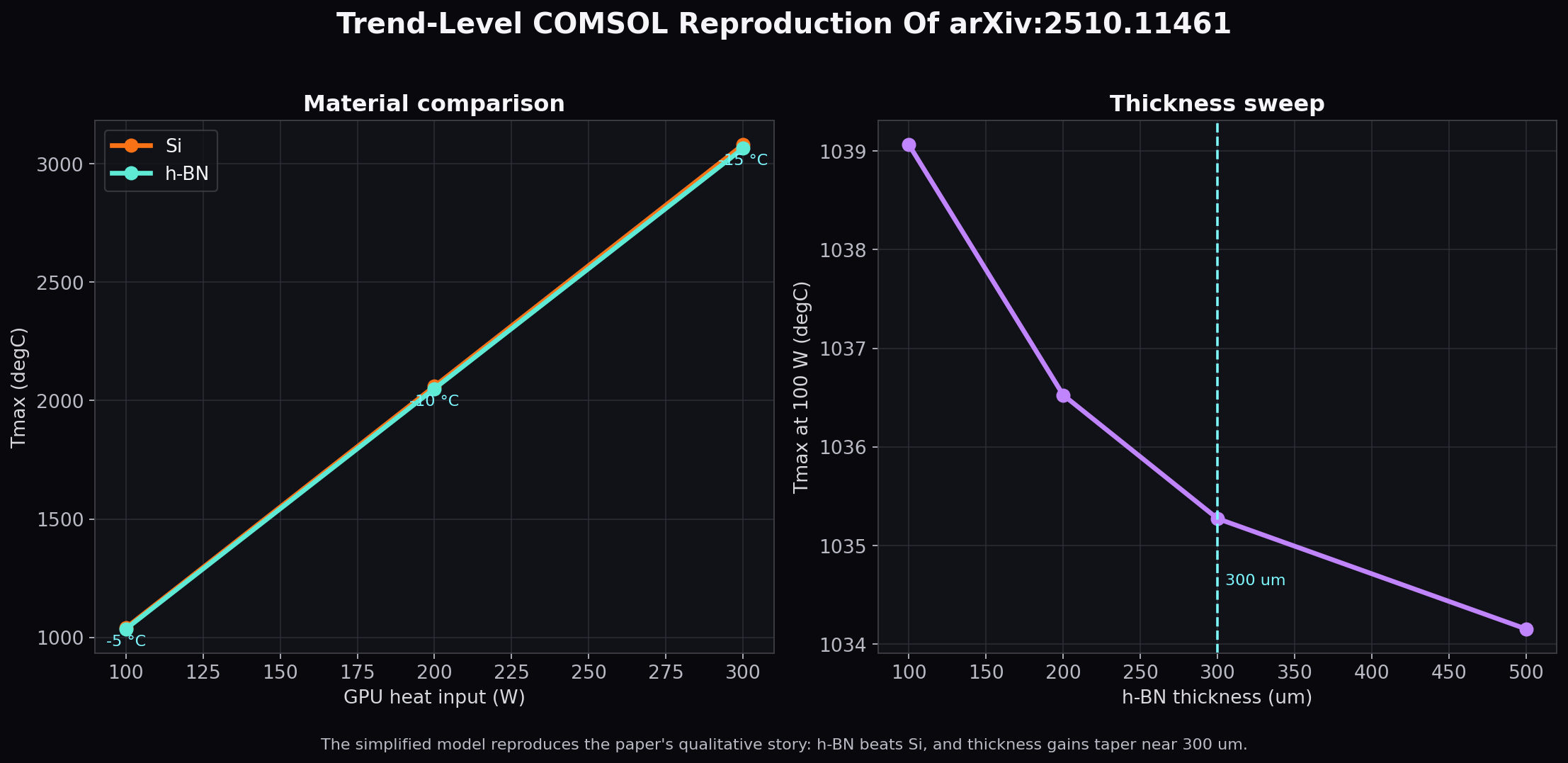
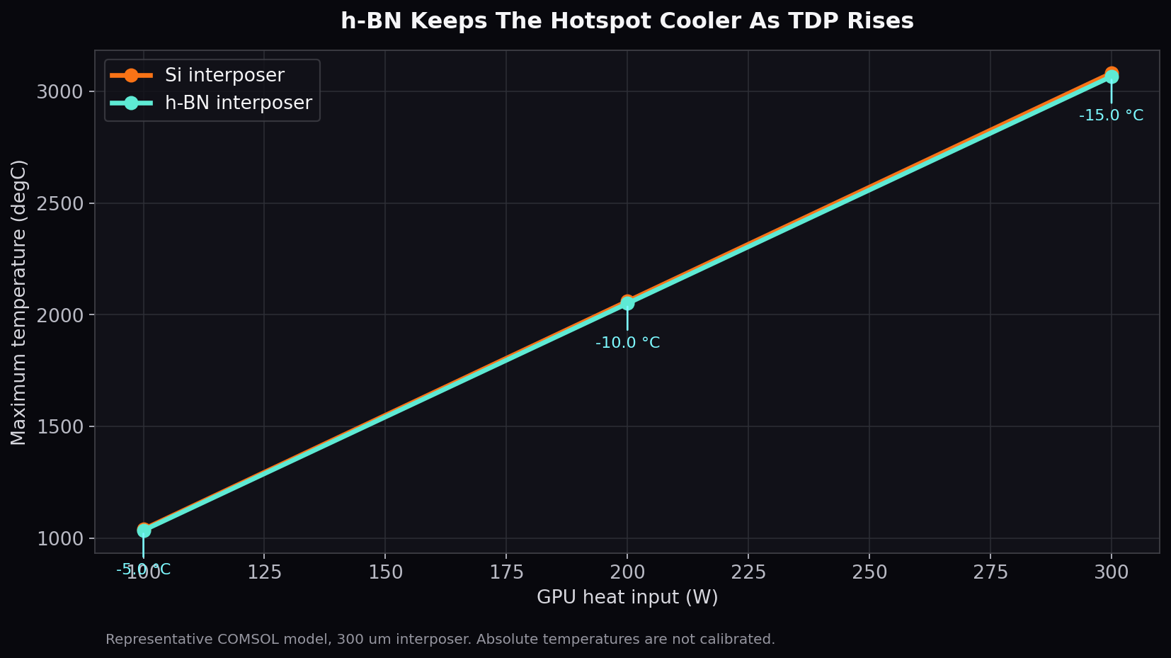
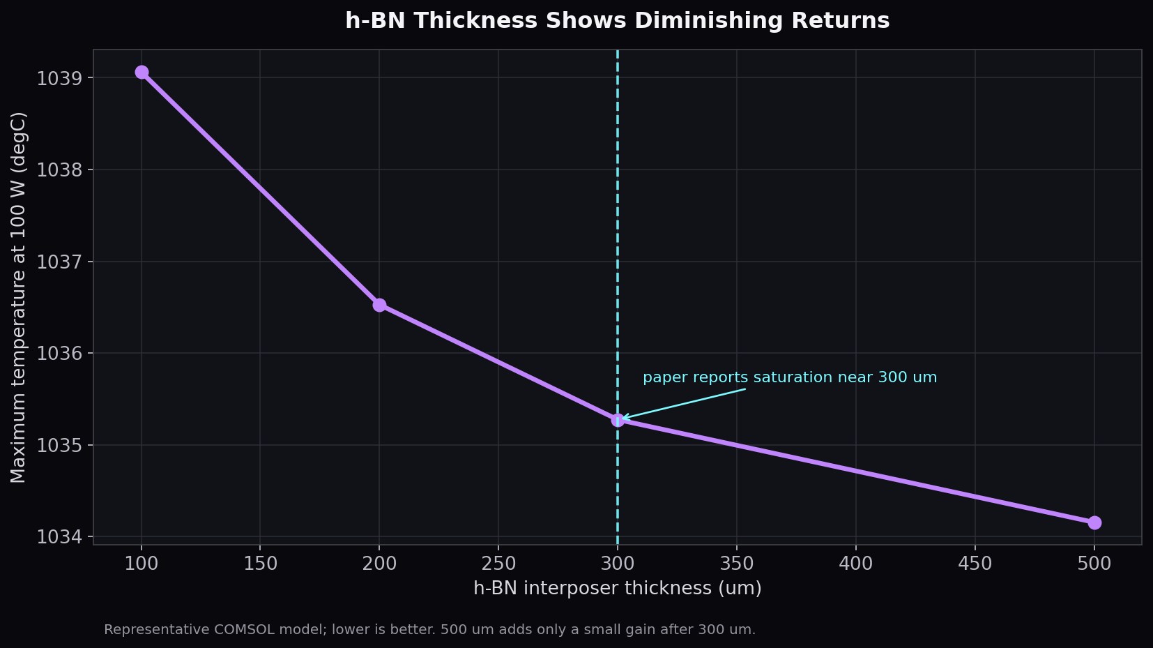
The absolute temperatures below are not calibrated acceptance numbers. They are high because this compact representative model applies the paper's 100/200/300 W load anchors to an assumed die and convection geometry. The acceptance signal is the trend: h-BN cooler than silicon, larger savings at higher power, and diminishing improvement around the 300 µm thickness region.

First Results

At 300 µm interposer thickness, h-BN reduced the hotspot temperature versus silicon in every TDP case:

Two-panel result figure showing h-BN versus silicon hotspot temperature by TDP and h-BN thickness sweep. — A compact view of the numeric result traces: material comparison on the left, h-BN thickness sweep on the right.

GPU Power	h-BN Tmax	Si Tmax	h-BN minus Si
100 W	1035.274 °C	1040.276 °C	-5.002 °C
200 W	2050.549 °C	2060.552 °C	-10.003 °C
300 W	3065.823 °C	3080.828 °C	-15.005 °C

The h-BN thickness sweep also moved in the same direction as the paper's reported thickness story: most of the gain appears by roughly 300 µm, with smaller improvement beyond it.

h-BN Thickness	Tmax at 100 W
100 µm	1039.062 °C
200 µm	1036.526 °C
300 µm	1035.274 °C
500 µm	1034.155 °C

Cropped COMSOL window after the TDP and h-BN thickness sweeps complete. — The working loop after multiple solves: selector files choose material, thickness, and power; the same COMSOL builder writes `.mph` checkpoints plus JSON/CSV result artifacts. The raw full capture keeps the Codex trace beside COMSOL.

Artifacts

The reproducibility bundle behind this post includes the assumptions, scripts, command trace, and numeric outputs. The heavy `.mph` checkpoints stayed in the internal work folder for now; the public assets below are enough to review and replay the agent side of the process.

paper assumptions CLI trace short demo video animated demo GIF GIF maker script video maker script identity script COMSOL builder script all results CSV sweep summary JSON TDP comparison plot thickness sweep plot

What Comes Next

The next reproduction layer is the HBM layout sweep: `20x1`, `10x2`, `5x4`, `4x5`, `2x10`, and `1x20`. That needs either author-supplied dimensions or a clearly documented surrogate for memory placement and TSV/interconnect paths. The harness is ready for that step because selections, material assignment, convection boundaries, solves, and numeric export are already repeatable.

The quiet lesson: the agent did not just write a COMSOL script. It had to choose the right control path, name the project, checkpoint early, inspect selections before assigning physics, catch a failed parameter expression, and keep the GUI visible enough for another human to follow.

COMSOL agent workflow: reproducing an HBM h-BN study with Codex.