A step-by-step walkthrough of building a complete COMSOL thermal model — geometry to results — with an AI agent at the controls.
// key takeaways
- The agent connects to a live COMSOL session — no copy-pasting code into Application Builder.
- It writes Python that calls COMSOL's Java API via JPype, executed in-process through
sim exec. - It sees the GUI via desktop screenshots, the same way a human looks at the screen.
- When something fails — a selection misses, a mesh has bad elements, the solver doesn't converge — the agent reads the error, diagnoses, and retries in the same session.
- The difference between "AI generates a script" and "AI drives the simulation" is the closed feedback loop: execute, observe, adapt.
Most attempts at using AI with COMSOL boil down to asking a chatbot to write methods, then copy-pasting them into Application Builder. That works for geometry scripting, but it breaks the feedback loop — the AI never sees the model, never catches errors visually, and can't iterate.
What if the agent could connect to a live COMSOL session, execute code, and see the GUI — the same way you would?
This post walks through exactly that: reproducing COMSOL Application Library model 847 (Heat Transfer in a Surface-Mount Package for a Silicon Chip) from scratch, with Claude at the controls.
The setup
sim is a lightweight runtime that connects AI agents to physics solvers. For COMSOL, it works like this:
The agent connects to a persistent COMSOL session. It can:
sim exec— send Python code that runs inside the live COMSOL modelsim screenshot— capture the server's desktop to see the COMSOL GUIsim inspect— query model state (materials, physics nodes, mesh stats)
No file round-tripping. No restarting COMSOL between steps. The model object stays in memory across all commands.
The model
A silicon chip in a plastic surface-mount package sits on an FR4 circuit board near a hot voltage regulator (50 °C). The chip dissipates ~20 mW. Copper thin layers provide heat spreading. Forced convection cools the exterior.
Goal: find the chip's maximum temperature and confirm it doesn't overheat.
Step 0: Connect to COMSOL
Claude starts a persistent session with the COMSOL GUI visible:
sim connect --solver comsol --ui-mode gui
COMSOL Desktop opens with a blank model. The agent now has a live handle to it.
Step 1: Create geometry
Claude sends 00_create_geometry.py via sim exec. The script builds:
- PC board (20 × 10 × 1 mm)
- Chip package body (9.9 × 3.9 × 0.2 mm)
- 16 gull-wing pins (L-shaped blocks, 8 per side)
- Silicon chip (3 × 1.5 × 0.1 mm)
- Work planes for ground plate and interconnect copper layers
The key code pattern — everything goes through COMSOL's Java API via JPype:
geom = model.component("comp1").geom().create("geom1", 3)
geom.lengthUnit("mm")

blk1 = geom.create("blk1", "Block")
blk1.set("size", JD([20.0, 10.0, 1.0]))
blk1.set("pos", JD([-10.0, -5.0, -1.9]))
blk1.label("PC Board")
# ... 16 pins, chip, work planes ...
geom.run("fin")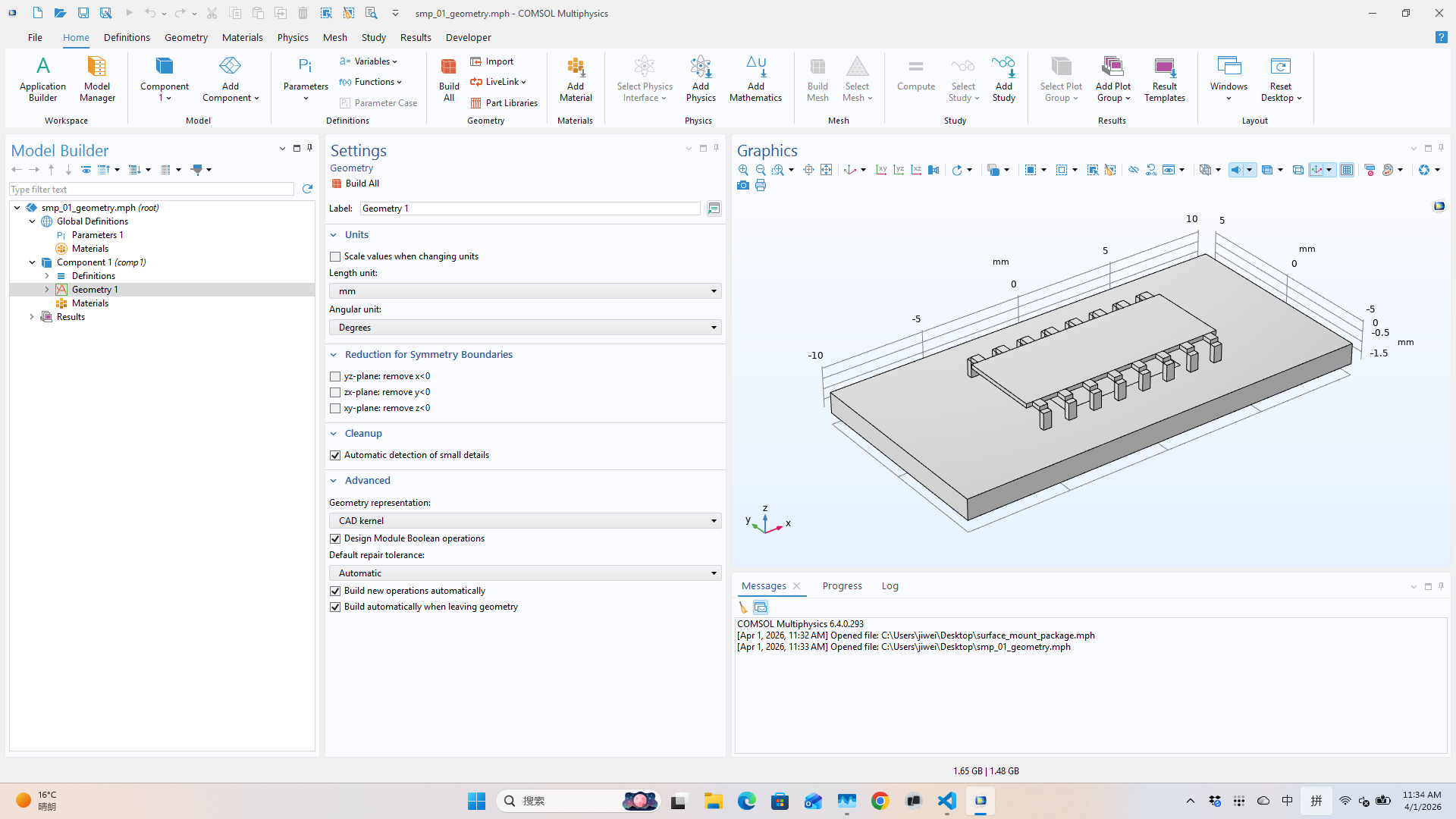
The agent can visually confirm the geometry looks right — all 16 pins present, chip centered on the package, board dimensions correct.
Step 2: Assign materials
Five materials, applied using Ball selections to identify each domain by position:
| Material | Domain | k (W/m·K) |
|---|---|---|
| Aluminum | All (pins are majority) | 237 |
| FR4 | Circuit board | 0.3 |
| Plastic | Package body | 0.2 |
| Silicon | Chip | 130 |
| Copper | Thin layer boundaries | 400 |
sel_chip = comp.selection().create("sel_chip", "Ball")
sel_chip.set("posx", "0"); sel_chip.set("posy", "0")
sel_chip.set("posz", "-0.05"); sel_chip.set("r", "0.01")

mat4 = comp.material().create("mat4", "Common")
mat4.label("Silicon")
mat4.selection().named("sel_chip")
mat4.propertyGroup("def").set("thermalconductivity", JS(["130[W/(m*K)]"]))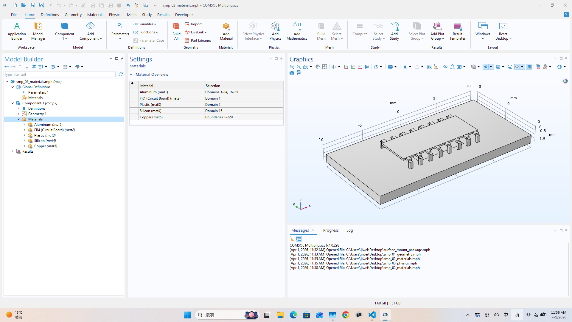
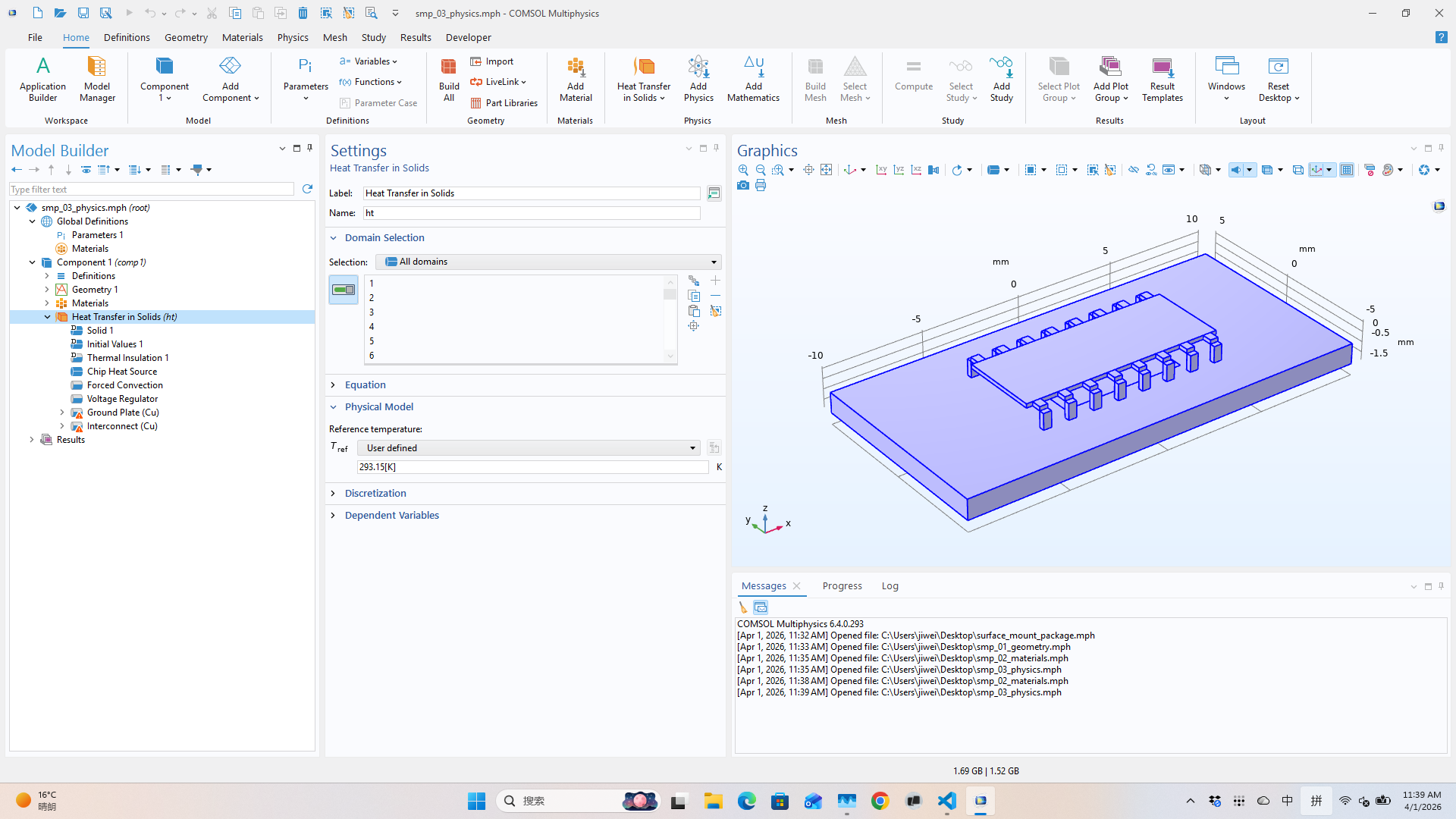
Step 3: Set up physics
Heat Transfer in Solids with five features:
- Heat source — 2×10⁸ W/m³ on the silicon chip (~20 mW total)
- Forced convection — h = 50 W/(m²·K), Tamb = 30 °C on all exterior surfaces
- Fixed temperature — 50 °C on the voltage regulator boundary
- Thin layer 1 — ground plate (copper, 0.1 mm)
- Thin layer 2 — interconnect trace (copper, 5 µm)
ht = comp.physics().create("ht", "HeatTransfer", "geom1")
hs1 = ht.create("hs1", "HeatSource", 3)
hs1.selection().named("sel_chip")
hs1.set("Q0", "2e8[W/m^3]")
The script includes a verification loop that prints how many entities each physics feature selected — the agent reads this output to confirm nothing was missed.
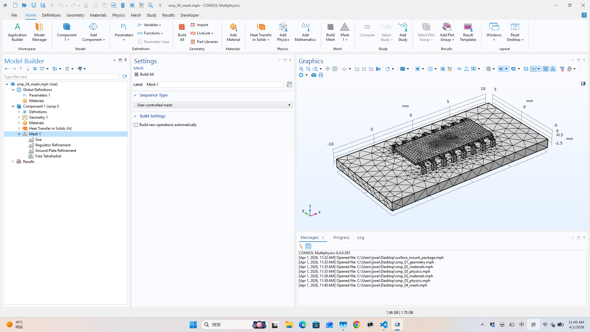
Step 4: Generate mesh
Fine global mesh with extra-fine refinement on the voltage regulator and ground plate boundaries:
mesh = model.component("comp1").mesh().create("mesh1")
mesh.autoMeshSize(jpype.JDouble(4))  # Fine
# ... local refinements ...
mesh.run()
The script reports element count and minimum quality. Claude reads these to verify mesh quality before solving.
Step 5: Solve
A stationary (steady-state) study — the solver typically finishes in under 10 seconds:
std = model.study().create("std1")
std.create("stat", "Stationary")
model.sol().create("sol1")
model.sol("sol1").createAutoSequence("std1")
model.sol("sol1").runAll()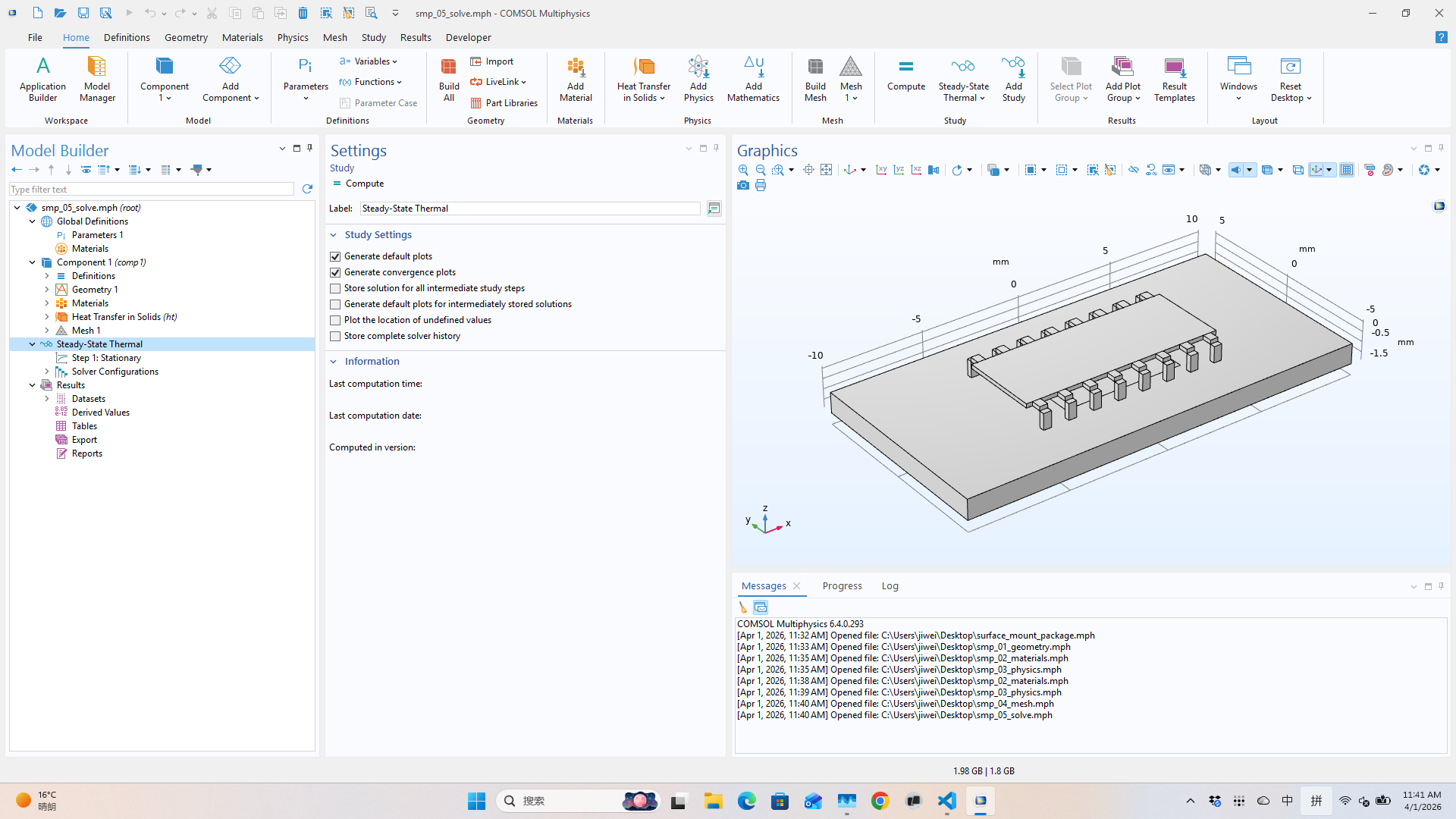
Step 6: Plot results
Three visualizations:
- Surface temperature — full assembly overview
- Temperature slices — ZX cross-sections through the package
- Chip surface detail — zoomed in on the silicon die
pg1 = res.create("pg1", "PlotGroup3D")
pg1.label("Temperature (Surface)")
s1 = pg1.create("surf1", "Surface")
s1.set("expr", "T"); s1.set("unit", "degC")
s1.set("colortable", "HeatCameraLight")
pg1.run()
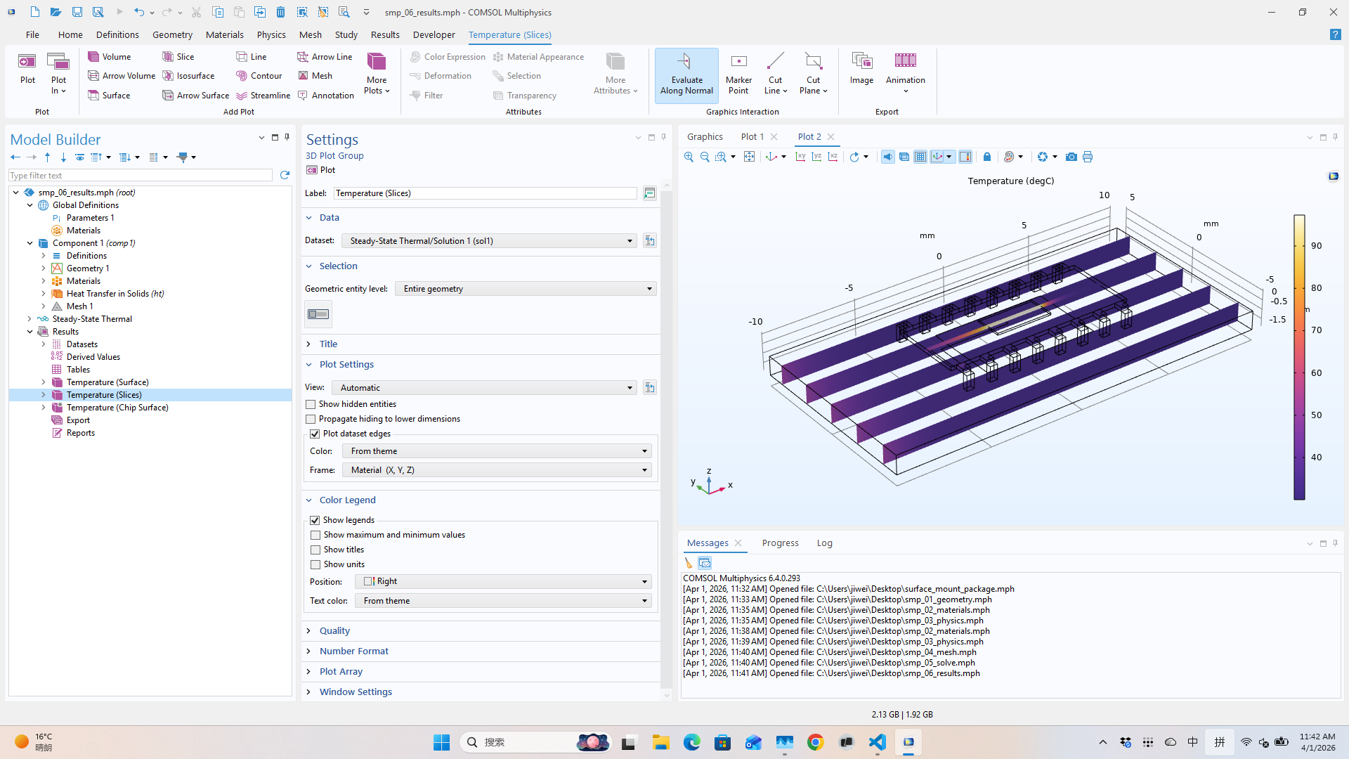
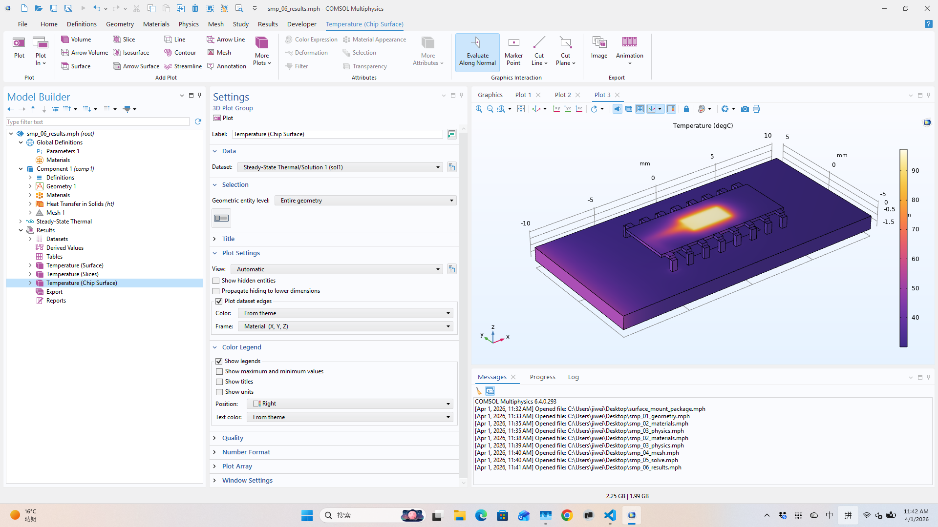
Result: chip max temperature ≈ 45.8 °C — the device does not overheat. (Reference value: 47.7 °C; the ~2 °C difference comes from simplified pin geometry.)
The agent loop
Every step above follows the same pattern:
- Claude decides what to do next (e.g., "create geometry").
- Claude writes a Python snippet using COMSOL's Java API (via JPype).
sim execsends the snippet to the running COMSOL process.- COMSOL executes it in-process — the model updates live.
sim screenshotcaptures the desktop so Claude can see the GUI.- Claude checks the screenshot, decides the next step.
- If something looks wrong, Claude writes a fix and re-executes.
No batch scripts. No copy-pasting into Application Builder.
No restarting COMSOL between steps. The model object
persists in memory across all
exec calls — Step 2 references geometry from
Step 1, Step 3 uses named selections from Step 2.
When things go wrong (and why that's the point)
The clean walkthrough above might suggest this is a one-shot process — write the script, run it, done. In practice, things fail. A Ball selection misses its target domain. A material property has the wrong units. A mesh operation fails because the geometry has a sliver face. The solver doesn't converge.
This is where the harness matters. When a step fails, the agent doesn't crash out — it reads the error, takes a screenshot to see the model state, diagnoses the problem, and sends a corrected snippet. The session is still alive. The model is still in memory. The agent just tries again.
For example, during development of this walkthrough:
- A pin union failed because two blocks didn't share a face — the agent adjusted the overlap and re-ran the geometry step.
- A Ball selection for the chip domain returned 0 entities — the agent checked the z-coordinate, realized the chip center was at −0.05 not 0.0, and fixed the selection radius.
- The mesh initially had poor-quality elements near thin pins — the agent added local refinement and re-meshed.
None of these required human intervention. The agent saw the failure, understood the cause, and fixed it — in the same live session.
This is the real difference between "AI generates a script" and "AI drives the simulation." Script generation is one-shot: it either works or you're back to debugging by hand. A harness gives the agent a closed feedback loop — execute, observe, adapt — the same loop a human engineer uses, just without the manual overhead.
What this enables
An agent with domain knowledge can drive the entire modeling workflow — geometry, materials, physics, meshing, solving, post-processing — writing API calls on the fly, adapting to whatever the problem requires. No pre-recorded methods or Application Builder macros needed.
The key insight: COMSOL's Java API is the automation interface, and JPype makes it callable from Python. Once you have that bridge and a runtime to manage the session, the agent has the same access to COMSOL that a human has through the GUI — including the ability to see what went wrong and try again.
Built with sim — the physics simulation runtime for AI agents. · Full cookbook: sim-cookbook / comsol / surface_mount_package